Audience

This series on Bloomberg Bquant is written for quants, software engineers, data analysts, and anyone trying to solve data engineering challenges with the Bloomberg stack.

There is not a lot of public, non-marketing technical information available on BQuant, Bloomberg’s development platform for data analysis. There’s no StackOverflow, few blog posts, case studies, etc. There’s also a fairly steep learning curve, either for new developers coding for the first time or seasoned developers learning the details of the stack.

I wrote this series with two users in mind: what I wish I had when I started using BQuant a few years ago and what my customers (analysts, quants, etc) need to know when they start using BQuant. My career is in software engineering, specializing in data engineering, so I may gloss over some of the technical points, and I may overgeneralize a few points when trying to write for a broad audience. This is the internet, so go ahead and criticize/comment/whatever.

Background

The world of Finance revolves around data, and among data providers Bloomberg reigns supreme (with competition, for sure). This post assumes familiarity with Bloomberg Terminal, and perhaps the Excel APIs (BDP/BDS/BDH/etc). If you’ve never used either, then this post is probably not for you.

Bloomberg introduced BQuant a few years ago, along with their new BQL API. In short, BQuant provides a Python programming environment letting a large range of analysts, quants and developers to do data stuff. I’ll talk a bit about why this is important in the next section.

Bloomberg’s BQuant has become our go-to tool for leveling up financial firms’ analytics capabilities. Whether we’re “modernizing” Excel-centric workflows or incorporating ML techniques, it all needs a home… and BQuant saves us the effort of having to build out a managed environment to operate it, along with sourcing data and providing ongoing platform maintenance. Bloomberg’s BQuant Enterprise service is both a programming environment and a “managed” service: you write Python¹ code that interacts with Bloomberg data via BQL². This environment is built on Jupyter³, a popular programming environment where you code in a Notebook comprised of Cells, each of which contains code (or markdown text). With BQuant Enterprise, you can schedule large tasks to run off-hours, cache large datasets and models to be shared across analysts, etc.

BQuant has two main variants:

• BQuant Desktop: runs on your computer alongside Terminal
• BQuant Enterprise: runs in the cloud

There are pros and cons to each of these. Bquant Enterprise is really the “full” product: generous data licensing, more horsepower, scheduling, centralized (AWS S3) storage, application development, and flexible custom environments. BQuant Desktop is limited and locked down: it runs in a “sandboxed” Python kernel, no “custom environments” (limited selection of packages), no user-user publishing, no git, data limits inherited from Terminal, etc. A lot of this is for the user’s protection: you don’t want a user running malicious code that can read from their desktop/etc. But, there are many cases where Desktop⁴ is the right solution.

BQuant - What?

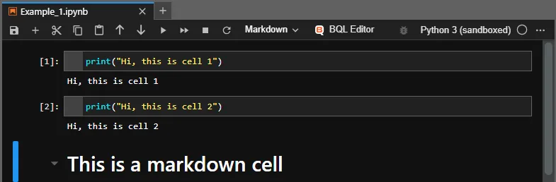Fig 1: Jupyter Cells

This post introduces you to a few of the basics of BQuant, including BQL, Jupyter Notebooks, Regressions in Python, and Plotly Charting.

Good, fast, cheap. Pick two

There’s an old engineering adage: “Good, fast, cheap. Pick two.”.

Spreadsheets are fast and cheap, accessible to many, but not necessarily good. Definitely not good for “data engineering”. Bloomberg provides its Excel APIs (BDP/BDH/BDS/etc, and now BQL). Spreadsheets are problematic for a few reasons:

• Fragile
• Not easily reusable
• No version control
• Complexity: It’s hard to
• Dreaded “#N/A Daily Capacity” data limits

Code is, well, not as cheap and is accessible to fewer developers, data analysts with training, and quants with programming chops. To get “fast” with code requires building with a purpose: building reusable components, putting the right team together, and having a clear vision to solve a class of problems, not just today’s problem. The result of a code-driven model can be transformative: imagine tweaking and deploying models in days, not weeks or months, testing new signals in minutes, with full accountability for every change.

Getting Started

Fire up bqnt bqnt<go>, start a new project, and let’s write something interesting.

In BQuant Enterprise, you’d also pick an Custom Environment (and optionally node type). We’ll cover this in BQuant [3], because the rest of my posts will assume certain things are already installed in a Custom Environment. For this post, it doesn’t matter.

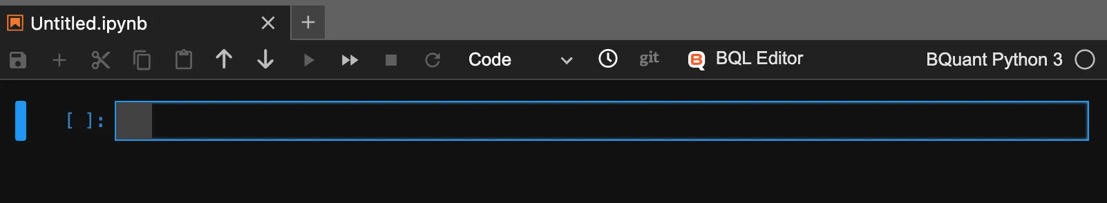
Empty Notebook

An empty project will launch with an blank “Untitled.ipynb”. This is an Interative PYthon NoteBook (ipynb). Code is organized in cells, which you can add using ”+“.

Every BQuant project has a default notebook:

Sharing and Collaborating

After you’ve written your code, you can “share” a copy of it or “publish” it with another Terminal user.

• Publishing lets other users run the code in Terminal. It’s a read-only interaction with the code.
• Sharing sends a complete copy to the other user, so they can edit it… but won’t see your subsequent edits.

We use Publish to share with non-coders and keep our project count low.

We avoid “sharing” because it creates full copies. Instead, we use git and manage our projects outside of BQuant. Even if you’re a team of 1, git is the way to go. If you think git is too complicated, just wait till you see what happens when you don’t use it.

* When you’re starting, it’s tempting to create one project per ipynb file. This leads to chaos; don’t do it. This does get a little challenging when you want to publish applications, which we’ll discuss in another post.

Final Thoughts before Code

For me, BQuant isn’t really about the coding platform. It’s about the ecosystem: access to the data, a fully managed application environment, collaboration, and reuse of code. This means we don’t need a large IT project to get started, and we don’t need to build out an entire stack from scratch.

All together, BQuant has sped up our development significantly. There was a fairly substantial ramp-up time* / learning curve: figuring out our development lifecycle and build/test lifecycle, along with creating a base platform and reusable components, was substantial. It has paid off: our team can focus on doing cool stuff with data, and our customers can rapidly consume and modify information in entirely new ways.

* I hope these posts will shorten this for you.

Let’s see the code

View this Notebook directly at: https://github.com/paultiq/bqnt_examples/blob/main/basics_p1.ipynb

All the data points here are fake / randomized.

# %package install plotly scikit-learn xgboost

import xgboost as xgb
import plotly.express as px
from sklearn.linear_model import LinearRegression
from sklearn.preprocessing import PolynomialFeatures
import pandas as pd

# Import packages used in this Notebook
import datetime
import bql

import plotly.io as pio

pio.renderers.default = "plotly_mimetype+notebook"
pio.templates["iqmo"] = pio.templates["plotly"]
pio.templates["iqmo"].layout.margin = dict(l=50, r=50, t=50, b=50)
pio.templates["iqmo"].layout.height = 250
pio.templates.default = "iqmo"

daterange = 29  # days
security = "IBM US Equity"

basics_query = f"""get(
      px_last
    ) for(
      ['{security}']
    ) with(
      dates=range(-{daterange}d, 0d),
      fill=prev,
      currency=USD
    )"""

bql_svc = bql.Service()

response = bql_svc.execute(basics_query)
base_df = bql.combined_df(response)

# Reset the index: bql's combined_df returns ID as a sole index.
base_df = base_df.reset_index()
base_df["date_ordinal"] = base_df["DATE"].apply(lambda x: x.toordinal())

px.line(base_df, x="DATE", y="px_last")

# Make a copy of the dataframe
df_withavgs = base_df.copy()

df_withavgs["sma_3day"] = df_withavgs["px_last"].rolling(3).mean()
px.line(df_withavgs, x="DATE", y=["px_last", "sma_3day"])

# This example uses scikit-learn (also called: sklearn) to perform a simple linear
# regression. This pattern of fitting a model, and then predicting, unlocks a lot of other tools
# You'll see xgboost uses the same flow.
# This model uses the entire date range, with no train/test split.

linear_model_full = LinearRegression()
X = df_withavgs[["date_ordinal"]]
y = df_withavgs["px_last"]

linear_model_full.fit(X, y)
df_withavgs["px_last_pred_fulltrain"] = linear_model_full.predict(X)

df_withavgs["sma_3day"] = df_withavgs["px_last"].rolling(3).mean()
px.line(df_withavgs, x="DATE", y=["px_last", "sma_3day", "px_last_pred_fulltrain"])

# This example uses scikit-learn (also called: sklearn) to perform a simple linear
# regression. This pattern of fitting a model, and then predicting, unlocks a lot of other tools
# You'll see xgboost uses the same flow.
# This model uses the entire date range, with no train/test split.

degree = 2  # quadratic
df_poly = df_withavgs.copy()

X = df_poly[["date_ordinal"]]
y = df_poly["px_last"]

poly = PolynomialFeatures(degree=degree)
X_poly = poly.fit_transform(X)

linear_model_poly = LinearRegression()
linear_model_poly.fit(X_poly, y)
df_poly["px_last_pred_poly"] = linear_model_poly.predict(X_poly)

px.line(df_poly, x="DATE", y=["px_last", "px_last_pred_fulltrain", "px_last_pred_poly"])

train_df = base_df.iloc[:21]
test_df = base_df[["DATE", "date_ordinal", "px_last"]].iloc[21:]

linear_model_split = LinearRegression()
X_train = train_df[["date_ordinal"]]
y_train = train_df["px_last"]

linear_model_split.fit(X_train, y_train)

X_test = test_df[["date_ordinal"]]
test_df["px_last_pred_split"] = linear_model_split.predict(X_test)

df_withpreds = pd.concat([train_df, test_df]).reset_index()
px.line(df_withpreds, x="DATE", y=["px_last", "px_last_pred_split"])

future_range = 14  # days
df_future = pd.DataFrame(
    {
        "date_ordinal": range(
            base_df["date_ordinal"].max() + 1,
            base_df["date_ordinal"].max() + future_range,
        )
    },
    index=range(base_df.index.max() + 1, base_df.index.max() + future_range),
)

X_future_pred = linear_model_full.predict(df_future)

df_future["px_last_pred_future"] = X_future_pred
df_future["DATE"] = pd.to_datetime(
    df_future["date_ordinal"].apply(lambda x: datetime.date.fromordinal(x))
)

df_with_future = pd.concat([df_withavgs, df_future])

px.line(
    df_with_future,
    x="DATE",
    y=["px_last", "px_last_pred_fulltrain", "px_last_pred_future"],
)

xg_df = base_df.copy()

xg_df["month"] = xg_df["DATE"].dt.month
xg_df["day_of_week"] = xg_df["DATE"].dt.dayofweek

train_df = xg_df.iloc[:-21]
test_df = xg_df.iloc[-21:]

X_train = train_df[["month", "day_of_week"]]
y_train = train_df["px_last"]

xmodel = xgb.XGBRegressor(
    n_estimators=100, learning_rate=0.1, objective="reg:squarederror"
)
xmodel.fit(X_train, y_train)

xg_df.loc[test_df.index, "xgpredicted_px_last"] = xmodel.predict(
    test_df[["month", "day_of_week"]]
)

px.line(xg_df, x="DATE", y=["px_last", "xgpredicted_px_last"])